

 Ashish Sharma
No money? No problem! Help us pay the cloud hosting bills without opening your wallet—just give
this ad link a click!😉💸
As digital products grow from handling a few hundred users to serving millions, databases inevitably face severe bottlenecks. Suddenly, simple queries stall, connection pools exhaust, and server CPU usage spikes to 100%. Throwing expensive hardware at the problem offers only temporary relief. True scalability requires deliberate architectural decisions.
Database optimization is not about applying a single magic trick. Instead, architects combine data layout strategies, intelligent caching, efficient network utilization, and algorithmic query tuning.
This guide breaks down the nine foundational database optimization techniques, explores real-world use cases, highlights critical trade-offs, and illustrates how these components integrate into a production-grade architecture.
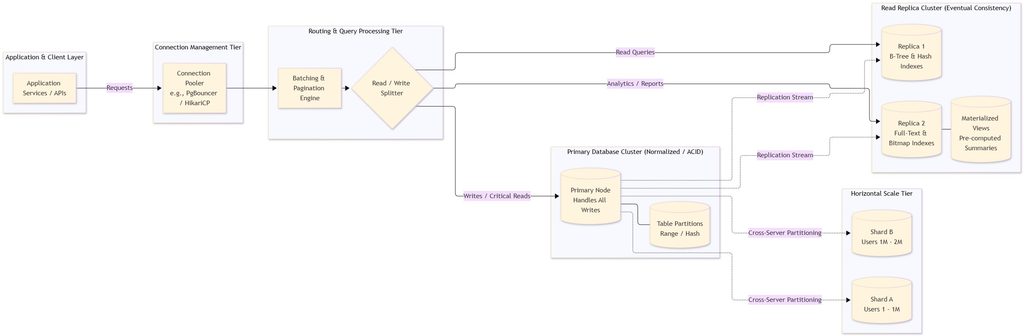
High-Level Architecture: End-to-End Database Optimization
The diagram below illustrates how modern systems layer these optimization techniques across the application, connection, and data tiers:
1. Database Replication: High Availability and Read Scalability
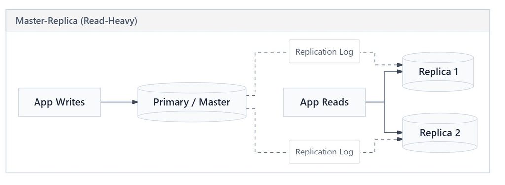
Replication duplicates database contents across multiple physical servers. Consequently, it transforms a single point of failure into a resilient, distributed system.
Architectural Models
- Primary-Replica (Master-Slave): A single primary node accepts all write operations (
INSERT,UPDATE,DELETE). Meanwhile, one or more read replicas asynchronously or synchronously mirror the changes and serve read traffic (SELECT). - Multi-Primary (Master-Master): Multiple nodes process both read and write queries simultaneously. While this model provides multi-region redundancy, it introduces complex write-conflict resolution logic.
Real-World Use Case
- E-Commerce Product Catalogs: Retail platforms like Amazon experience read-to-write ratios often exceeding 20:1. Customers browse millions of product pages (reads) while only a fraction place orders (writes). Routing catalog browsing to read replicas prevents shopping carts from locking up the primary database.
- Disaster Recovery: Maintaining a live replica in another geographic availability zone ensures immediate automated failover if a primary data center suffers an outage.
2. Sharding vs. Partitioning: Scaling Massive Datasets
When tables grow to hundreds of millions of rows, single disks and query engines choke. Engineers employ partitioning and sharding to divide massive datasets into manageable slices.
| Dimension | Table Partitioning | Database Sharding |
|---|---|---|
| Location | Single database server / instance | Distributed across multiple physical servers |
| Mechanism | Logical split managed by database engine | Physical split often managed by application/proxy |
| Complexity | Low (transparent to application queries) | High (requires distributed joins, shard keys) |
| Primary Goal | Optimize disk scan speed and maintenance | Overcome hardware, memory, and CPU ceilings |
Partitioning Strategies (Single Instance)
- Range Partitioning: Groups records by continuous boundaries (such as date ranges or order values).
- Example: Storing audit logs into monthly partitions (
logs_2026_01,logs_2026_02). The query engine scans only the current month’s partition during incident investigations.
- Example: Storing audit logs into monthly partitions (
- Hash Partitioning: Applies an algorithm (e.g.,
hash(user_id) % num_partitions) to scatter records uniformly. Consequently, this eliminates hot spots on write-heavy tables.
Sharding Across Servers (Horizontal Scaling)
Sharding assigns distinct server clusters to subsets of data using a chosen Shard Key.
- Example: A global SaaS application shards user data by tenant ID or country code. European customers reside entirely on European database instances, while North American data resides in Virginia. This layout boosts query speed and satisfies regional compliance requirements (e.g., GDPR).
3. The CAP Theorem: Balancing Consistency and Performance
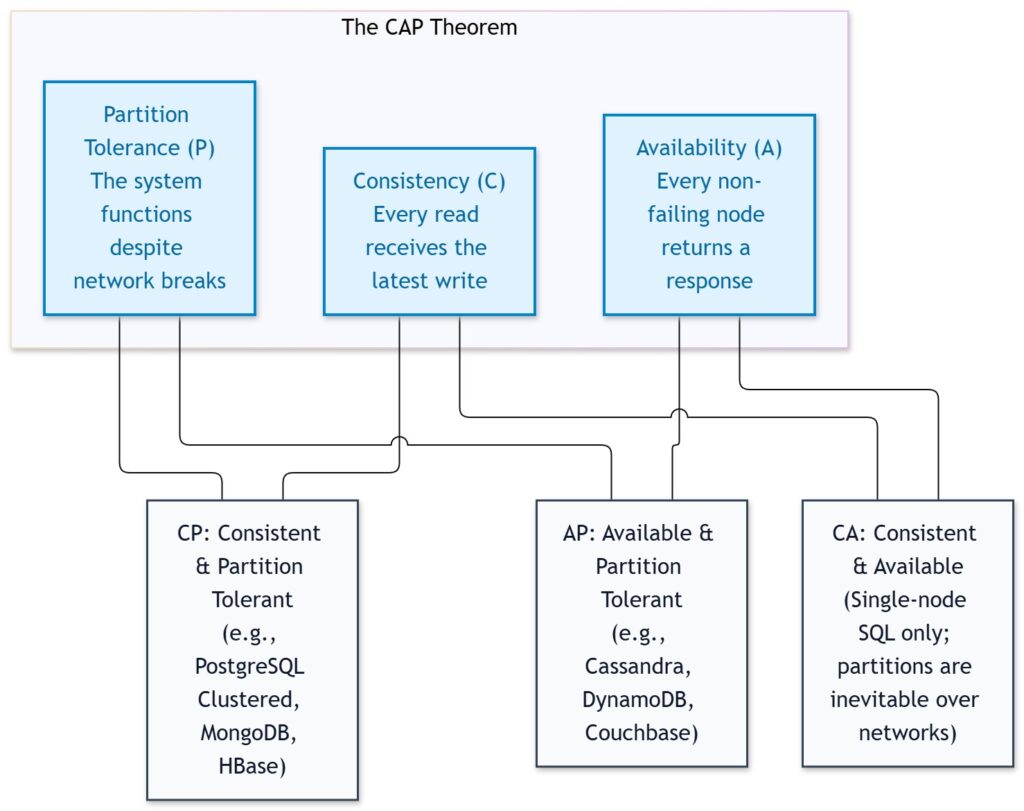
Distributed database architects inevitably confront the CAP Theorem, which states that a distributed system can simultaneously guarantee only two out of three characteristics during network failures:
- Consistency (C): Every read returns the most recent write.
- Availability (A): Every non-failing node returns a response, without guaranteeing it is the freshest version.
- Partition Tolerance (P): The system survives communication delays or dropped messages between nodes.
The Performance Trade-off
Because network partitions (P) are inevitable in modern cloud environments, architects must choose between CP and AP.
- Choosing Consistency (CP): Financial ledger systems block transactions if replicas fail to synchronize immediately. As a result, writes take longer, and network hiccup events cause requests to fail rather than record incorrect balances.
- Choosing Availability (AP): Social media platforms prioritize throughput. When a creator uploads a post, millions of followers can view it seconds apart across different continents. Embracing eventual consistency eliminates locking overhead, delivering lightning-fast response times.
4. Indexing Strategies: Accelerating Data Retrieval
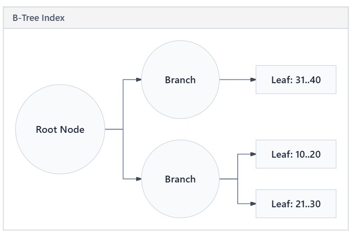
An index is a specialized data structure that helps the query engine locate records without scanning the entire table. However, indexes introduce a hidden trade-off: faster reads directly penalize write performance. Every INSERT, UPDATE, or DELETE forces the database to rebalance index trees.
Common Index Types and Use Cases
- B-Tree Indexes: The universal default. They organize data hierarchically, making them ideal for equality searches (
WHERE id = 500) and range comparisons (WHERE created_at BETWEEN '2026-01-01' AND '2026-02-01'). - Hash Indexes: Use internal hash maps. They provide blazing O(1) lookups for strict equality (
WHERE email = 'user@domain.com'), but fail on sorting or range conditions. - Full-Text Indexes: Parse text documents into inverted word tokens. For instance, e-commerce product search bars use full-text indexing to match queries like
"wireless noise-canceling headphones". - Bitmap Indexes: Map distinct values to bit arrays. They perform best on low-cardinality columns (such as
status = 'ACTIVE' | 'PENDING' | 'CANCELLED') in reporting and data warehousing platforms.
5. Normalization vs. Denormalization: Integrity vs. Read Speed
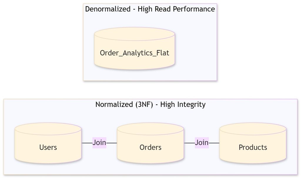
Database modeling revolves around a fundamental tension: eliminating duplicate data versus minimizing expensive join operations.
When to Normalize
Normalized schemas (typically Third Normal Form or 3NF) split entities into distinct, well-related tables.
- Benefits: Zero data redundancy, minimal storage footprints, and total immunity to data update anomalies.
- Best Fit: Core banking engines, ERP systems, and transactional backbones where record accuracy is paramount.
When to Denormalize
Denormalization strategically duplicates related fields into a single table, eliminating multi-table joins.
- Benefits: A single query fetches all necessary fields in one fast sequential scan.
- Trade-offs: Updates require updating multiple records, increasing storage costs and inconsistency risks.
- Best Fit: High-speed mobile feed APIs and business analytics platforms.
Modern Best Practice: Adopt a hybrid architecture. Maintain a strictly normalized transactional primary database (OLTP) for mutations, and continuously project data into denormalized read views or search engines (OLAP) for fast retrieval.
6. Connection Pooling: Eliminating Handshake Overhead
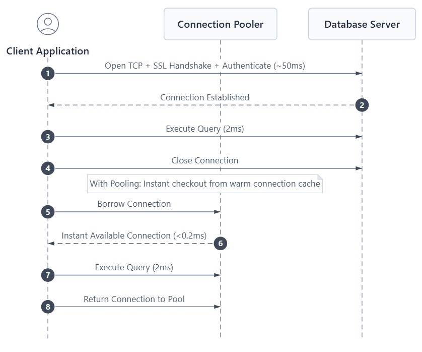
Opening a database connection is an expensive, multi-step process: TCP handshakes, TLS negotiation, authentication verification, and operating system memory allocation.
How Connection Pooling Works
A connection pooler (e.g., HikariCP for Java, PgBouncer for PostgreSQL) keeps a set of warm, pre-authenticated connections ready in memory. When an application thread needs data, it borrows a connection, executes the query, and returns it immediately.
Pool Sizing Guidelines
Counterintuitively, setting connection pools too high harms database throughput. Hundreds of concurrent active connections trigger heavy CPU context-switching and disk I/O contention.
A proven empirical baseline for PostgreSQL sizing is:
Pool Size = (CPU Cores×2) + Disk Spindle Count
7. Query Optimization: Doing Less Work Per Query
Hardware upgrades cannot compensate for poorly authored queries. High-performance engineering requires reducing disk scans, memory buffers, and network round trips.
1. Defeating the N+1 Query Problem
The issue occurs when an application loads a collection of parent records and then runs individual child queries for every row:
-- Inefficient: 1 query + N child queries
SELECT * FROM orders WHERE user_id = 10; -- returns 100 rows
SELECT * FROM order_items WHERE order_id = 1;
SELECT * FROM order_items WHERE order_id = 2; -- (repeats 100 times!)
Optimized Approach: Use eager joins or batch fetches:
-- Optimized: Single round trip
SELECT o.id, o.order_date, i.item_name, i.price
FROM orders o
INNER JOIN order_items i ON o.id = i.order_id
WHERE o.user_id = 10;
2. Inspecting the Execution Plan (EXPLAIN ANALYZE)
Always verify how the query planner processes your SQL. Look out for Seq Scan (Full Table Scan) on large tables, nested loop joins on unindexed columns, and expensive sorting operations that spill into temporary disk files.
8. Materialized Views: Precomputing Heavy Aggregations
Standard database views recalculate their underlying queries on every request. In contrast, a Materialized View executes complex multi-table joins and calculations once, persisting the physical result directly onto disk.

Practical Example
Consider an analytics dashboard displaying daily revenue per region across 50 million transaction rows:
CREATE MATERIALIZED VIEW daily_regional_revenue AS
SELECT
    region_id,
    DATE(created_at) AS sale_date,
    SUM(total_amount) AS daily_revenue
FROM sales_transactions
GROUP BY region_id, DATE(created_at);- Performance Impact: Instead of aggregating millions of rows on every user page load (taking 5-10 seconds), the dashboard reads the materialized table in under 5 milliseconds.
- Refresh Strategies: Refresh views periodically during off-peak hours using
REFRESH MATERIALIZED VIEW CONCURRENTLY, which allows users to read existing data while the view recalculates in the background.
9. Batching and Pagination: Controlling Data Flow
Processing data in unconstrained volumes exhausts memory buffers, triggers network timeouts, and locks database pages. Batching and pagination impose strict limits on data operations.
Batching for Write Workloads
Inserting 50,000 sensor readings one by one forces 50,000 separate network round trips and transaction commits. Grouping inserts into batches of 1,000 reduces transaction overhead by up to 90%:
-- Batch Insert: One round trip, single commit block
INSERT INTO sensor_telemetry (sensor_id, reading, recorded_at) VALUES
(101, 24.5, NOW()),
(102, 26.1, NOW()),
(103, 23.9, NOW());
Keyset (Cursor) Pagination for Read Workloads
Traditional offset pagination (LIMIT 20 OFFSET 500000) forces the database to read and discard half a million records before returning 20 rows. Keyset pagination relies on indexed columns to skip historical data instantaneously:
-- Slow: Discards 500,000 rows
SELECT * FROM activities ORDER BY id ASC LIMIT 20 OFFSET 500000;

-- Fast: Index seek directly to the next cursor
SELECT * FROM activities WHERE id > 500000 ORDER BY id ASC LIMIT 20;
Architectural Decision Framework
The following matrix summarizes when to deploy each optimization technique based on your operational bottleneck:
| Optimization Technique | Primary Bottleneck Solved | Read vs. Write Impact | Primary Trade-off |
|---|---|---|---|
| Replication | High read load, single server outages | Massive read boost | Write overhead; replication lag |
| Partitioning | Large table scan overhead | Faster targeted scans | Partition management overhead |
| Sharding | Hardware CPU, memory, and disk ceilings | Scales both reads & writes | Complex distributed queries & transactions |
| Indexes | Full table scans on specific filters | Drastically speeds up reads | Degrades write and update speeds |
| Denormalization | High-cost relational joins | Drastically speeds up reads | Data duplication; risk of stale records |
| Connection Pooling | Handshake latency & connection limits | Boosts overall throughput | Requires proper tuning to avoid starvation |
| Query Optimization | Slow algorithms, excessive I/O | Reduces execution time | Requires active code profiling & maintenance |
| Materialized Views | Repetitive heavy aggregate functions | Sub-millisecond reads | Periodic data staleness between refreshes |
| Batching / Pagination | Memory spikes & payload bloat | Optimizes throughput | Slightly higher batch assembly latency |
Conclusion
Scaling databases is an ongoing balancing act between consistency, throughput, latency, and operational complexity.
Begin by eliminating basic inefficiencies: configure connection pooling, fix the N+1 query problem, and add selective B-tree indexes. As traffic builds, distribute read queries across replication clusters and introduce materialized views for heavy analytics. Finally, implement horizontal sharding and eventual consistency only when your data volumes outgrow single-server infrastructure. By applying these optimization strategies incrementally, you ensure your database architecture remains performant, resilient, and cost-effective.